

In my previous blog, we pulled back the curtain to discuss what a Distributed Control System is and how it works. We looked at the major pieces and how they replace hundreds of relays and miles of pipes and wires. Now that we’ve seen the components, let’s look at how they manage to pack all that functionality into a tiny little box.
All Distributed Control Systems (DCSs) are centered around one key component: the microprocessor. The microprocessor, first invented in 1971, was a significant advancement from using transistors and simple integrated circuits to process individual electrical signals. (Betker, Fernando, & Whalen, 1997)
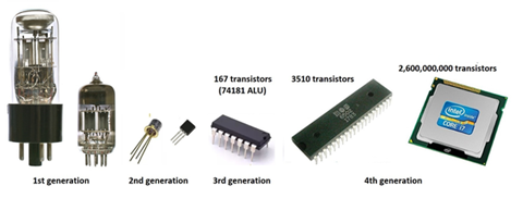
Basically, a microprocessor controls the direction and magnitude of a LOT of electrical signals. All computers work by controlling the flow of electrical signals. As technology has improved, the ability to put more control into a smaller device has driven us from the Sci-Fi movie room-sized computers to the newest smartwatch. Microprocessors have made it possible to have more technological power on your wrist than we used to take us to the moon!
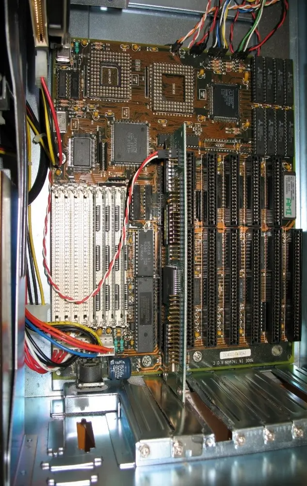
One microprocessor can’t do the job alone, it takes multiple processors to perform all the complicated tasks in a major control system, and those are usually attached to “cards” and installed in “racks.” The racks typically connect the cards to the data highway and to their power supply through what is called “the backplane.” So how do these tiny little data managers allow you to start a pump from 5 miles away? You have to speak their language.
Computers are stupid. No, I don’t mean in the way your grandfather calls computers stupid, I mean computers literally only know two words. Yes and No. They are so stupid in fact, they don’t even know the words, yes and no, they only know the numbers 1 and 0. This is referred to as “binary” language or code. The use of binary can get much more complicated than we want to talk about here. In a nutshell, someone (the computer expert) has to tell the computer what every 1 and 0 means, and what to do with that information. They have to write the “code.” This is no simple task, not only for the person writing the code but for the person working with the code later on. Just to provide an example, the ORIGINAL Oregon Trail game contained over 800 lines of code!
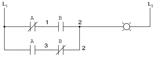
Thankfully, most interactions with control system programming don’t involve knowing how to read code. Instead, controls are typically programmed using what is called “Ladder Logic,” a graphical way of representing the code, that emulates an electrical schematic. The two “rails” (L1 and L2) are the inlet power and the output, and the “rungs” are the control circuits. (Kuphaldt, Chapter 6 LADDER LOGIC, n.d.)
When it comes to describing the language used in programming a controls system, remember that the processor takes an input, and YOU have to tell it what to do with that input to get the desired output. This is accomplished in ladder logic by the use of “gates.” A gate is basically the processor’s way of taking a number of inputs, figuring out what they mean, and giving the desired output. It is important to remember that in microprocessor controls, there is always an “output” either 1 or 0 (often referred to as true or false).
Some common gates are shown here:
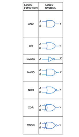
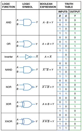
Remember, the language of a microprocessor is in 1 or 0 (yes or no, true or false); so the circuit is always speaking. The gate takes the input and converts those 1’s and 0’s into a single yes or no output. For example, An AND gate will only give you a 1 if both inputs are 1. The OR gate will give you a 1 as long as either input contains a 1. This replaces physical contacts in a circuit that would have to close to energize the relay, motor, alarm, etc.
Based on the inputs, logic gates can have several combinations of results. These are summarized by writing up “truth tables.” A truth table is a method of charting the possible inputs into the gate, and what the output would be. This is extremely helpful when looking at larger programs that use multiple gates.
Using a simple ladder logic diagram, let’s see what the logic gate and its truth table look like.
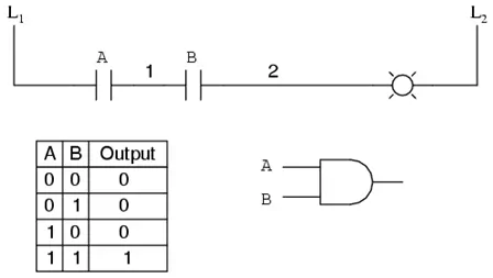
As you can see from our setup, “contacts” A and B both have to close to make the lamplight. To add realism, let’s assign components to our diagram. Contact “A” will represent a closed detector on a breaker, contact “B” will represent an “Open” valve position detector (VPD) and the light will represent a pump ready indicator on a DCS screen.
Looking at the truth table, if power is not available (A = 0) and the VPD does not show open (B=0) the “pump ready” indicator will be out (the circuit says NO). If the power is unavailable, and the VPD indicates open, the indicator stays out, vice versa, if power is available, but the VPD doesn’t show open, the indicator stays out. However, if power is available (A=1) AND the VPD indicates “Open” (B=1) then the gate output is 1 (the circuit says YES) and the “pump ready” indicator is activated.
This is just a simple example to introduce ladder logic and logic diagrams. When a programmer builds the controls into a PLC or DCS, they use ladder logic. This language gives the microprocessor the ability to take little 1’s and 0’s from all over the plant and provide functions such as auto-starts, alarms, and even more complicated operations (like Boiler Level Control). The logic diagrams (showing the gates) are the meat of the software functions and can get quite confusing. In my next blog, we will take a more complicated logic diagram and break it down step by step.
Betker, M. R., Fernando, J. S., & Whalen, S. P. (1997). The history of the microprocessor. Bell Labs Technical Journal, 2(4), 29-56. Retrieved 8 26, 2021, from http://beatriceco.com/bti/porticus/bell/pdf/bell_labs_journals/bell_labs_technical_journal_autumn_1997_3.pdf
Kuphaldt, T. R. (2003, May). Lessons in Electric Circuits – Volume IV. Retrieved August 26, 2021, from IBIBLIO.ORG: http://www.ibiblio.org/kuphaldt/electricCircuits/Digital/DIGI_6.html
Kuphaldt, T. R. (n.d.). Chapter 6 LADDER LOGIC. Retrieved 8 26, 2021, from http://www.ibiblio.org/kuphaldt/electricCircuits/Digital/DIGI_6.html